Cohort Approach For Customer Lifetime Value (LTV) Calculation

Saturday. February 10, 2018 - 8 mins

I hope you all read my previous post where I tried to understand a general LTV concept. Now let’s begin our investigation how to calculate LTV if we have enough historical data (at least, 1 year). Let’s remind us a general LTV formula from the previous post:

$$\text{ Customer LTV = } \text{R}_0 * \text{AGMPU}_0 + \text{R}_1 * \frac{\text{AGMPU}_1}{\text{ (1 + d)}^1} + \text{ ...} + \text{R}_n * \frac{\text{AGMPU}_n}{\text{ (1 + d)}^n} + \text{ ... } \qquad \text{ (1) } \\\ \text{where} \\\ \text{d - discount rate, i.e. the interest rate you can get if you put your money in the bank } \\\ \text{R}_n \text{ – cohort retention rate in month n (e.g 100 % in the 0th month, 35 % in the 1st month, etc.) } \\\ \text{ AGMPU}_n \text{ – average gross margin per user in month n (e.g. 5 bucks in the 0th month, 11 bucks in 1st month, etc.) }$$

The algorithm for calculating LTV via a cohort approach is the following:

1. Calculate historical retention rates and AGMPU for cohorts (of course, if you have historical data, otherwise, use this approach).
2. Calculate average historical retention rates and AGMPU weighted on cohorts’ sizes.
3. Fit statistical models for retention rates and AGMPU versus a cohorts lifespan.
4. Predict retention rates and AGMPU for the future using created models (ideally, you will find such an exponential function for a retention rate that it will go to zero after some lifetime).
5. Calculate LTV using formula (1)

Historical retention and AGMPU

I use the dataframe cdnowElog from BTYD package for my calculations (you could find the R code I wrote here). After the first manipulations the data looks like that:

cust	date	price	birth	period
1	1997-01-01	29.33	1997-01-01	0
1	1997-01-18	29.73	1997-01-01	0
1	1997-08-02	14.96	1997-01-01	7
…	…	…	…	…

Cust, date and price were in the initial dataset. What I did is calculate the birth field (a starting month for every cohort a customer belongs to) and the period (how many months passed from the first order of a customer). Then I did some GroupBy work and got all the historical values I needed (remind: you could find the whole code here). The first 3 rows look like that:

birth	period	retained_users	revenue	orders	cohort_size	retention	agmpu
1997-01-01	0	781	28592.70	1.13	781	1.00	10.98
1997-01-01	1	124	7003.73	1.45	781	0.16	16.94
1997-01-01	2	95	4241.64	1.38	781	0.12	13.39
…	…	…	…	…	…	…	…

At this point I got the historical data about all cohorts:

• Retained users – how many members from the initial cohort made an order in the i-th period.
• Revenue – sum of the revenue by all cohorts members.
• Orders – average number of orders per cohort member in i-th period.
• Cohort size – initial cohort size.
• Retention - proportion of cohorts members who made an order in the i-th period.
• AGMPU - average gross margin per user in the i-th period (if you want to find a more detailed definition of this, please look my previous post).

Average historical retention rates and AGMPU

At this stage we need to calculate an average (weighted by a cohort size to pay more attention to big cohorts) of everything we got on the previous one by the period:

period	avg.retention	avg.agmpu	avg.orders
0	1.00	12.07	1.17
1	0.15	15.24	1.39
2	0.12	13.17	1.30
…	…	…	…

Statistical models for retention rates and AGMPU

Here we reach the most interesting part: modeling our average retention and average AGMPU (I’m not touching average orders here, just leave it here to show that we could calculate a lot of different metrics by cohort). What we need to do now is investigate the behavior of average retention and average AGMPU relatively to the cohort period and find the mathematical function which explains it the best. Firstly we should just create two plots:

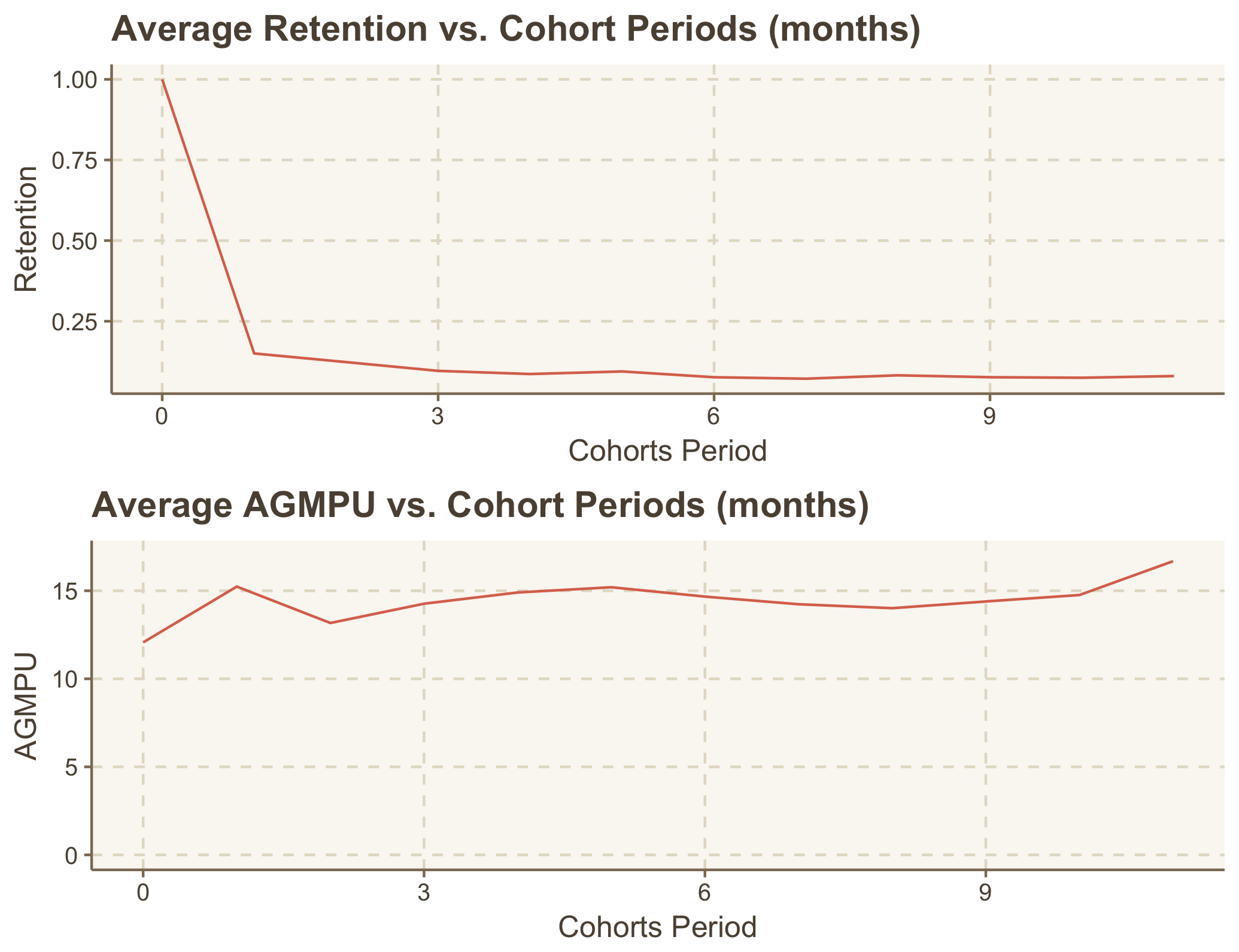
This data doesn’t look perfect, I know. But I still could see the patterns common to these metrics: some kind of an exponential decay of the retention and the growth of AGMPU over the cohort lifetime. And it seems quite logical to me: the most users who used your service once will stop using it after the first try and the users who continued to use your service will likely pay more because they will use it more.

The next important step is to select appropriate math functions to fit these variables. Regarding the retention, the answer is quite obvious: people usually use the exponential decay. I personally use the mix of two exponential decays:

$$f(period) = a * e^{-\text{b } * \text{ period}} + (1 - a) * e^{-\text{c } * \text{ period}}$$

How to fit AGMPU is the less obvious question. As for me, I use the following function (you also could use ln(x)):

$$f(period) = \frac{\text{a} * \text{period + b}}{\text{period + c}}$$

When you’ve chosen appropriate functions, it’s time to evaluate constants a, b, c minimizing the sum of squared errors between the actual target values and predicted ones:

$$\sum_{i=1}^{N} (y_i - f_i(period))^2 \rightarrow \min\limits_{a, b, c} \\\ \text{where} \\\ \text{y – actual metric values (retention or AGMPU)} \\\ \text{f – predicted metric values (retention or AGMPU)}$$

If it accidentally sounds complicated, then just imagine that we try to decrease our errors’ sum above by looking at different combination of our constants a, b, c.

After finding optimal a, b, c and plotting resulted predictions, we get:

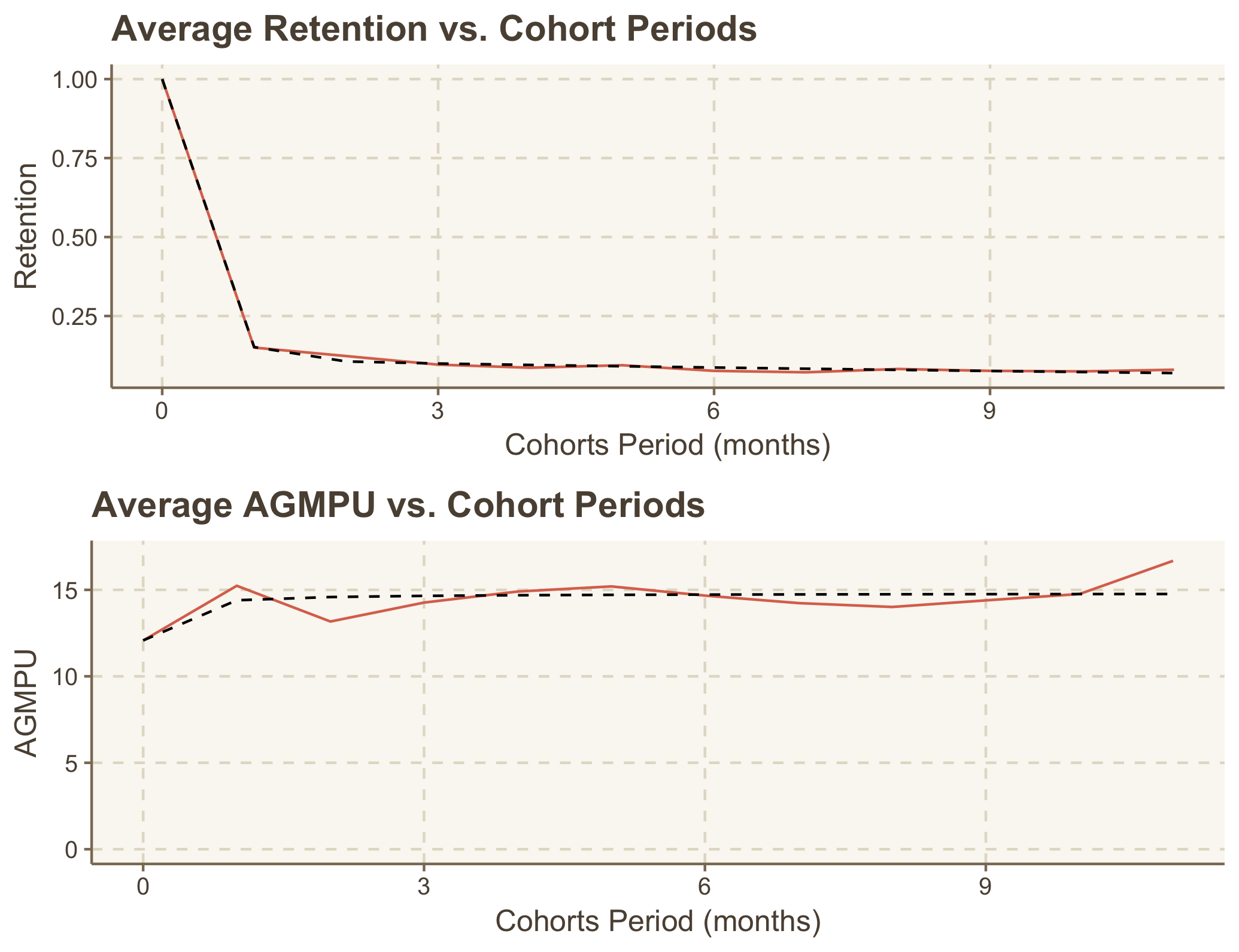
Retention rates and AGMPU prediction

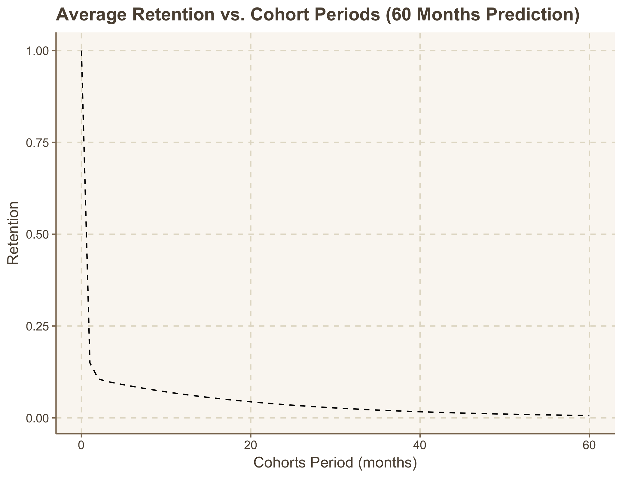
After we’ve fitted our retention and AGMPU, let’s choose the period we’re going to predict LTV for. Often this is quite clear: you just predict your retention for the next 5-10 years and usually you could see that the retention rate goes very close to zero from some point. In that case we just limit our LTV period when the retention rate first touch values close to zero. If we predict our retention for 5-10 years and see that a cohort doesn’t decay completely, then we need to decide how to limit the LTV calculation period. It should suits our calculation goal, often it’s enough just to know when our cohort becomes profitable.

In the case of my dataset, I can see that the cohort disappears after 5 years:

LTV calculation

Finally we’re ready to calculate LTV. We just sum predicted AGMPU multiplied by retention rate and divided by discount rate for every cohort’s life period (in my case 5 years). As a result I got that an average user from my dataset brings $40,06 of lifetime profit to the company.

How you can use this result?

• Check that your customer acquisition costs (CAC) are not higher than your customer LTV. It’s common to say that your ratio LTV:CAC should be from 3:1. But if it’s not lower than 1:1, then… At least, you don’t waste your money completely.
• Calculate LTV by different marketing channels. You can find that some of your campaigns are just useless while others really attract wealthy customers.
• Check the period when your customers’ sum of returns (used for LTV calculation) first becomes above CAC. This is your profitability period.

That’s all I wanted to share. If you have any questions or corrections, feel free to write a comment.

Tweet Share

comments powered by Disqus