Statistical comparison of two means

Thursday. March 29, 2018 - 6 mins

One common example of statistical hypotheses testing is means comparison. Imagine that you’re analyzing results of a survey about the dependence of gender and wage. All you want to know is whether any difference in average wages exists or not. Let’s illustrate this case with the data of the survey Wages, Experience and Schooling. Its results contain data about hourly wages (in dollars of 1980) of males and females in USA in 1980.

> library(data.table)
> dt <- fread('https://raw.githubusercontent.com/vincentarelbundock/Rdatasets/master/csv/Ecdat/Wages1.csv')
> head(dt)
   exper    sex school     wage
1:     9 female     13 6.315296
2:    12 female     12 5.479770
3:    11 female     11 3.642170
4:     9 female     14 4.593337
5:     8 female     14 2.418157
6:     9 female     14 2.094058

The first thing you can do is to calculate average wages for females and males correspondingly:

> dt[, .(avg_wage=mean(wage, na.rm=TRUE)), by='sex']
      sex avg_wage
1: female 5.146924
2:   male 6.313021

However, you couldn’t just compare these numbers and make a conclusion from it. No! Firstly, you need to understand what the population you want to make a conclusion about. In our case we’re dealing with two populations – males and females in USA. However, we don’t have the data about the whole population. All we have is our survey data which presents just two samples containing randomly selected men and women in USA. We’re using samples as an approach to investigate populations. When we calculate a sample mean, we use it only as an estimation of a population mean. This estimation has an error, i.e. actually a population mean lies in the interval (sample mean - error, sample mean + error). This is called a confidence interval.

What are the confidence intervals?

Firstly, we need to familiarize ourselves with probably two most important theorems in the world of scientific research: Law of Large Numbers (LLN) and Central Limit Theorem (CLT). The latter one is actually a set of theorems, but it doesn’t matter for now. I will present you a brief overview of them but if you want to get a deeper understanding, watch this.

Law of Large Numbers (LLN)
This theorem tells us that if we have a sample with a number of observations approaching to the infinity (in practice, we should have at least 30 observations) then a sample mean $\bar x$ is a good approximation of a population mean $μ$ :

\begin{equation} \bar X_n \to μ \text{ as } n \to \infty \text{ with the probability = 1} \end{equation}

Central Limit Theorem (CLT)
Imagine that we have some distribution (doesn’t matter which exactly!) with known $μ$ (population mean) and $\sigma^2$ (variance). We construct a lof of samples from this distribution with size $n$ and calculate all sample means $\bar x_1, \bar x_2, ..., \bar x_n , ..., \bar x_k$ , then this new random variable of sample means $\bar X_n$ will follow Normal distribution with population mean $μ$ and variance $\frac{\sigma^2}{n}$ :

\begin{equation}
\bar X_n \sim N(μ, \frac{\sigma^2}{n})
\end{equation}

If we standardize $\bar X_n$ , then we get the following:

\begin{equation}
\frac{\bar X_n - μ}{\sigma / \sqrt{n}} \sim N(0, 1)
\end{equation}

This will allow us to use the properties of Standard Normal distribution:

Confidence Interval

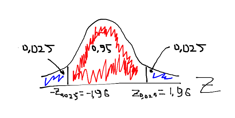
On the picture above we could see Z-score (or technically standard normal distribution). We know everything about this distribution and especially that 95 % of distribution’s values vary between -1.96 and 1.96. Stop. Does it mean that 95 % of values of our random variable $\frac{\bar X_n - μ}{\sigma / \sqrt{n}}$ also lie in the range [-1.96, 1.96]? Yes, exactly! Let’s write this in a more statistical way:

\begin{equation}
P(-1.96 \leq \frac{\bar X_n - μ}{\sigma / \sqrt{n}} \leq 1.96) \\
P(\frac{-1.96 \sigma}{\sqrt{n}} \leq \bar X_n - μ \leq \frac{1.96 \sigma}{\sqrt{n}}) \\ P(\bar X_n - \frac{1.96 \sigma}{\sqrt{n}} \leq μ \leq \bar X_n + \frac{1.96 \sigma}{\sqrt{n}}) \end{equation}

So, it means that the actual mean $μ$ with 95 % probability will lie in the interval $\bar X_n \pm \frac{1.96 \sigma}{\sqrt{n}}$ . If we want to get the interval at another percent of confidence, e.g. 99 % or 90 %, we just need to get the corresponding Z-value.

Calculation

Cool, we understand the concept of confidence intervals. Let’s come back to our example of comparing wages of males and females in USA. We’ve already calculated means so now we just can use what we’ve learned or not? Practically yes, but there is one detail we need to take into account. We don’t know anything about males’ or females’ wage distribution except our sample. It means that we don’t know neither $μ$ neither $\sigma$ . In this case people use a sample variance ( $S^2$ ) as an approximation of a population variance ( $\sigma^2$ ) and a t-statistic instead of a z-statistic. Why a t-statistic? Because t-distribution converges to Normal distribution when a sample size is big enough and it has fatter tails when a sample size is small (n < 30): this makes it more reliable for an estimation of confidence intervals and prevents its underestimation.

The final formula for the confidence interval for $μ$ we’re going to use will be the following:

\begin{equation}
\bar X_n \pm \frac{t_{1-\frac{\alpha}{2}} S}{\sqrt{n}} \\ \text{where} \\ t_{1-\frac{\alpha}{2}} \text{ – t-statistic value for } 1-\frac{\alpha}{2} \text{ percent of confidence,} \\ \alpha \text{ – a level of the tolerable error,} \\ S \text{ – sample standard deviation.}
\end{equation}

We have rather big samples for both males and females, so in our case a t-statistic value for 95 % confidence interval will be very close to 1.96 (see the table). What’s next? We need to calculate the sample size and the sample standard deviation for both males and females’ wages:

> table(dt$sex) # sample size
female   male 
  1569   1725 
  
> dt[, .(std_wage=sd(wage, na.rm=TRUE)), by='sex'] # standard deviation
      sex std_wage
1: female 2.876237
2:   male 3.498861

Finally we can calculate the confidence intervals:

\begin{equation}
μ_{female} \in [5.15 - \frac{1.96 * 2.88}{\sqrt{1569}}, 5.15 + \frac{1.96 * 2.88}{\sqrt{1569}}] \\ μ_{female} \in [5, 5.29] \\ \end{equation}

\begin{equation}
μ_{male} \in [6.31 - \frac{1.96 * 3.5}{\sqrt{1725}}, 6.31 + \frac{1.96 * 3.5}{\sqrt{1725}}] \\ μ_{male} \in [6.15, 6.48] \\ \end{equation}

R code for these calculations:

means <- dt[, .(avg_wage=mean(wage, na.rm=TRUE)), by='sex']
n <- table(dt$sex) # sample size
stds <- dt[, .(std_wage=sd(wage, na.rm=TRUE)), by='sex'] # standard deviation

# confidence interval
female_low <- means[sex == 'female']$avg_wage + qt(0.025, n['female']) * (stds[sex == 'female']$std_wage / sqrt(n['female']))
female_high <- means[sex == 'female']$avg_wage + qt(0.975, n['female']) * (stds[sex == 'female']$std_wage / sqrt(n['female']))
male_low <- means[sex == 'male']$avg_wage + qt(0.025, n['male']) * (stds[sex == 'male']$std_wage / sqrt(n['male']))
male_high <- means[sex == 'male']$avg_wage + qt(0.975, n['male']) * (stds[sex == 'male']$std_wage / sqrt(n['male']))

Conclusion

Okay, now we see that average wages for males and females are really different because confidence intervals do not have intersections. We see that with a probability 95 % the average wage for females varies from 5 to 5.29 while for males – from 6.15 to 6.48. We can conclude that on average males earned 22.5 % more than females in USA in 1980.